
First steps#
Welcome! On this page we will guide to you through the first steps required to start working with hopsy!
Installation#
hopsy is available on PyPI, so you may just install using
pip install hopsy
From source#
If instead, you want to build hopsy from source, you need to download the code from GitHub or juGit
git clone https://jugit.fz-juelich.de/IBG-1/ModSim/hopsy --recursive # or
git clone https://github.com/modsim/hopsy --recursive
and either compile a binary wheel using
pip wheel --no-deps . -w dist
or use CMake
mkdir hopsy/cmake-build-release && cd hopsy/cmake-build-release
cmake ..
make
Note however, that the former approach allows you to install the compiled binary wheel using
pip install dist/hopsy-x.y.z-tag.whl
Polytope sampling in a nutshell#
Convex polytope sampling considers the problem of sampling probability densities \(f\) supported on a linearly constrained space, i.e. a convex polytope
with \(A \in \mathbb{R}^{n \times d}, b \in \mathbb{R}^n\). Such probability densities can arise for example when performing Bayesian inference on ODE systems, most prominently in metabolic flux analysis [1]_. Often, those probability densities are not analytically tractable and, thus, we need to resort to numerical sampling tools like Markov chain Monte Carlo simulations. hopsy offers a variety of different samplers for this exact purpose. Moreover, hopsy aims to be a general
purpose sampling library by leveraging the abstract formulation of the polytope sampling problem given earlier. Finally, since polytope sampling remains an open problem with new methods being developed as we speak, hopsy also allows to implement custom sampling algorithms.
Sampling from a simplex#
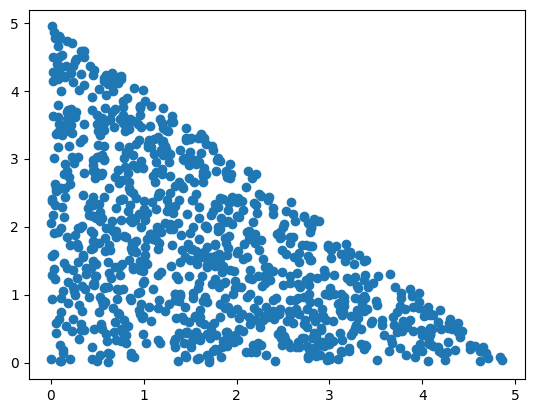
In hopsy, the target density we aim to sample from is defined by a hopsy.Problem, which takes the A matrix and b vector defining the linear inequality constraints, as well as model object. For starters, we will drop the model object, in which case we will be sampling the uniform density on \(\mathcal{P}\), which in the upcoming example is a simplex:
[4]:
import hopsy
import matplotlib.pyplot as plt

problem = hopsy.Problem(A=[[1, 1], [-1, 0], [0, -1]], b=[5, 0, 0])

chain = hopsy.MarkovChain(problem, starting_point=[.5, .5])
rng = hopsy.RandomNumberGenerator(seed=42)

accrate, samples = hopsy.sample(chain, rng, n_samples=1000, thinning=10)

plt.scatter(samples[:,:,0], samples[:,:,1])
plt.show()
Sampling a custom-implemented truncated standard Gaussian#
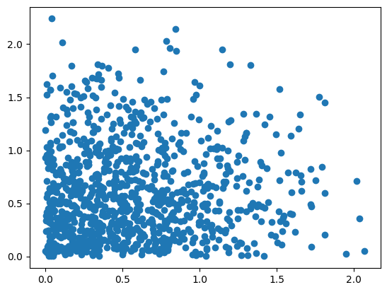
In hopsy, a model is any Python-object implementing at least a log_density function, which has to implement a (possibly unnormalized) probability density \(f\).
[5]:
class StandardGaussian:
    def log_density(self, x):
        return -x.dot(x)

problem = hopsy.Problem(A=[[1, 1], [-1, 0], [0, -1]], b=[5, 0, 0],
                        model=StandardGaussian())

chain = hopsy.MarkovChain(problem, starting_point=[.5, .5])
rng = hopsy.RandomNumberGenerator(seed=42)

accrate, samples = hopsy.sample(chain, rng, n_samples=1000, thinning=10)

plt.scatter(samples[:,:,0], samples[:,:,1])
plt.show()
Sampling with a custom sampler#
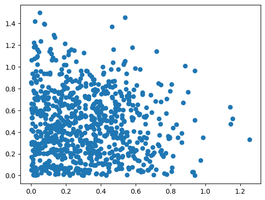
For demonstration purposes, we next try to sample previous distribution by a sampler which proposes new states from a cube. In the easiest case, a proposer only needs to implement a propose method. For non-symmetric proposal distributions, a log_acceptance_probability method needs to be provided as well. This is covered in more in-depth in our sampling user guide.
[6]:
class CubeProposal:
    uniform = hopsy.Uniform(-1, 1)
    def propose(self, rng):
        return [self.state[0] + self.uniform(rng), self.state[1] + self.uniform(rng)]

chain = hopsy.MarkovChain(problem, proposal=CubeProposal, starting_point=[.5, .5])
rng = hopsy.RandomNumberGenerator(seed=42)

accrate, samples = hopsy.sample(chain, rng, n_samples=1000, thinning=10)

plt.scatter(samples[:,:,0], samples[:,:,1])
plt.show()
Footnotes